Note
Click here to download the full example code
Example: Predicting COVID-19 patients outcome using MRCs
In this example we will use MRCpy.MRC and MRCpy.CMRC to predict the outcome
of a COVID-19 positive patient at the moment of hospital triage. This example
uses a dataset that comprises different demographic variables and biomarkers of
the patients and a binary outcome Status where Status = 0
define the group of survivors and Status = 1 determines a decease.
The data is provided by the Covid Data Saves Lives initiative carried out by HM Hospitales with information of the first wave of the COVID outbreak in Spanish hospitals. The data is available upon request through HM Hospitales here .
See also
For more information about the dataset and the creation of a risk indicator using Logistic regression refer to:
[1] Ruben Armañanzas et al. “Derivation of a Cost-Sensitive COVID-19 Mortality Risk Indicator Using a Multistart Framework” , in 2021 IEEE International Conference on Bioinformatics and Biomedicine (BIBM), 2021, pp. 2179–2186.
First we will see how to deal with class imbalance when training a model using
syntethic minority over-sampling (SMOTE) techniques. Furthermore, we will
comparetwo MRC with two state of the art machine learning models probability
estimation . The selected models are CMRC(phi = 'threshold' ,
loss = 'log') & MRC(phi = 'fourier' , loss = 'log') for the group of
MRCs and Logistic Regression (LR) & C-Support Vector Classifier(SVC) with the
implementation from Scikit-Learn.
# Import needed modules
import matplotlib.pyplot as plt
import numpy as np
import pandas as pd
import seaborn as sns
from imblearn.over_sampling import SMOTENC
from sklearn import preprocessing
from sklearn.linear_model import LogisticRegression
from sklearn.metrics import (
    classification_report,
    confusion_matrix,
    ConfusionMatrixDisplay,
)
from sklearn.model_selection import train_test_split
from sklearn.svm import SVC

from MRCpy import CMRC, MRC
COVID dataset Loader:
def load_covid(norm=False, array=True):
    data_consensus = pd.read_csv("data/data_consensus.csv", sep=";")
    # rename variables
    variable_dict = {
        "CD0000AGE": "Age",
        "CORE": "PATIENT_ID",
        "CT000000U": "Urea",
        "CT00000BT": "Bilirubin",
        "CT00000NA": "Sodium",
        "CT00000TP": "Proth_time",
        "CT0000COM": "Com",
        "CT0000LDH": "LDH",
        "CT0000NEU": "Neutrophils",
        "CT0000PCR": "Pro_C_Rea",
        "CT0000VCM": "Med_corp_vol",
        "CT000APTT": "Ceph_time",
        "CT000CHCM": "Mean_corp_Hgb",
        "CT000EOSP": "Eosinophils%",
        "CT000LEUC": "Leukocytes",
        "CT000LINP": "Lymphocytes%",
        "CT000NEUP": "Neutrophils%",
        "CT000PLAQ": "Platelet_count",
        "CTHSDXXRATE": "Rate",
        "CTHSDXXSAT": "Sat",
        "ED0DISWHY": "Status",
        "F_INGRESO/ADMISSION_D_ING/INPAT": "Fecha_admision",
        "SEXO/SEX": "Sexo",
    }
    data_consensus = data_consensus.rename(columns=variable_dict)
    if norm:  # if we want the data standardised
        x_consensus = data_consensus[
            data_consensus.columns.difference(["Status", "PATIENT_ID"])
        ][:]
        std_scale = preprocessing.StandardScaler().fit(x_consensus)
        x_consensus_std = std_scale.transform(x_consensus)
        dataframex_consensus = pd.DataFrame(
            x_consensus_std, columns=x_consensus.columns
        )
        data_consensus.reset_index(drop=True, inplace=True)
        data_consensus = pd.concat(
            [dataframex_consensus, data_consensus[["Status"]]], axis=1
        )
    data_consensus = data_consensus[
        data_consensus.columns.difference(["PATIENT_ID"])
    ]
    X = data_consensus[
        data_consensus.columns.difference(["Status", "PATIENT_ID"])
    ]
    y = data_consensus["Status"]
    if array:
        X = X.to_numpy()
        y = y.to_numpy()
    return X, y
Addressing dataset imbalance with SMOTE
The COVID dataset has a significant problem of class imbalance where the
positive outcome has a prevalence of 85% (1522) whilst the negative outcome
has only 276. In this example oversampling will be used to add syintetic
records to get an almost balanced dataset. SMOTE (Synthetic minority
over sampling) is a package that implements such oversampling.
X, y = load_covid(array=False)
described = (
    X.describe(percentiles=[0.5])
    .round(2)
    .transpose()[["count", "mean", "std"]]
)
pd.DataFrame(y.value_counts().rename({0.0: "Survive", 1.0: "Decease"}))
So we create a set of cases syntehtically using 5 nearest neighbors until
the class imbalance is almost removed. For more information about
SMOTE refer to it’s documentation .
We will use the method SMOTE-NC for numerical and categorical variables.
See also
For more information about the SMOTE package refer to:
[2] Chawla, N. V., Bowyer, K. W., Hall, L. O., & Kegelmeyer, W. P. (2002). SMOTE: synthetic minority over-sampling technique. Journal of artificial intelligence research, 16, 321-357.
# We fit the data to the oversampler
smotefit = SMOTENC(sampling_strategy=0.75, categorical_features=[3])
X_resampled, y_resampled = smotefit.fit_resample(X, y)
described_resample = (
    X_resampled.describe(percentiles=[0.5])
    .round(2)
    .transpose()[["count", "mean", "std"]]
)
described_resample = described_resample.add_suffix("_SMT")
pd.concat([described, described_resample], axis=1)
We see how the distribution of the real data and the resampled data is different. However the distribution between classes is kept similar due to the creation of the synthetic cases through 5 nearest neighbors.
pd.DataFrame(
    y_resampled.value_counts().rename({0.0: "Survive", 1.0: "Decease"})
)
Probability estimation
In this section we will estimate the conditional probabilities and analyse
the distribution of the probabilities depending on the real outcome . The
probability estimation is better when using loss = log. We use
CMRC(phi = 'threshold', loss = 'log') and
MRC(phi = 'fourier' , loss = 'log'. We will then compare these MRCs
with SVC and LR with default parameters.
Load classification function:
These function classify each of the cases in their correspondent confusion matrix’s category. It also allows to set the desired cut-off for the predictions.
def defDataFrame(model, x_test, y_test, threshold=0.5):
    """
    Takes x,y test and train and a fitted model and
    computes the probabilities to then classify in TP,TN , FP , FN.
    """
    if "predict_proba" in dir(model):
        probabilities = model.predict_proba(x_test)[:, 1]
        predictions = [1 if i > threshold else 0 for i in probabilities]
        df = pd.DataFrame(
            {
                "Real": y_test.tolist(),
                "Prediction": predictions,
                "Probabilities": probabilities.tolist(),
            }
        )
    else:
        df = pd.DataFrame(
            {"Real": y_test.tolist(), "Prediction": model.predict(x_test)}
        )
    conditions = [
        (df["Real"] == 1) & (df["Prediction"] == 1),
        (df["Real"] == 1) & (df["Prediction"] == 0),
        (df["Real"] == 0) & (df["Prediction"] == 0),
        (df["Real"] == 0) & (df["Prediction"] == 1),
    ]
    choices = [
        "True Positive",
        "False Negative",
        "True Negative",
        "False Positive",
    ]
    df["Category"] = np.select(conditions, choices, default="No")
    df.sort_index(inplace=True)
    df.sort_values(by="Category", ascending=False, inplace=True)
    return df
Train models:
We will train the models with 80% of the data and then test with the other 20% selected randomly.
X_train, X_test, y_train, y_test = train_test_split(
    X_resampled, y_resampled, test_size=0.2, random_state=1
)

clf_MRC = MRC(phi="fourier", use_cvx=True, loss="log").fit(X_train, y_train)
df_MRC = defDataFrame(model=clf_MRC, x_test=X_test, y_test=y_test)
MRC_values = pd.DataFrame(df_MRC.Category.value_counts()).rename(
    columns={"Category": type(clf_MRC).__name__}
)
MRC_values["Freq_MRC"] = MRC_values["MRC"] / sum(MRC_values["MRC"]) * 100

clf_CMRC = CMRC(phi="threshold", use_cvx=True, loss="log").fit(
    X_train, y_train
)
df_CMRC = defDataFrame(model=clf_CMRC, x_test=X_test, y_test=y_test)
CMRC_values = pd.DataFrame(df_CMRC.Category.value_counts()).rename(
    columns={"Category": type(clf_CMRC).__name__}
)
CMRC_values["Freq_CMRC"] = CMRC_values["CMRC"] / sum(CMRC_values["CMRC"]) * 100

clf_SVC = SVC(probability=True).fit(X_train, y_train)
df_SVC = defDataFrame(model=clf_SVC, x_test=X_test, y_test=y_test)
SVC_values = pd.DataFrame(df_SVC.Category.value_counts()).rename(
    columns={"Category": type(clf_SVC).__name__}
)
SVC_values["Freq_SVC"] = SVC_values["SVC"] / sum(SVC_values["SVC"]) * 100

clf_LR = LogisticRegression().fit(X_train, y_train)
df_LR = defDataFrame(model=clf_LR, x_test=X_test, y_test=y_test)
LR_values = pd.DataFrame(df_LR.Category.value_counts()).rename(
    columns={"Category": type(clf_LR).__name__}
)
LR_values["Freq_LR"] = (
    LR_values["LogisticRegression"]
    / sum(LR_values["LogisticRegression"])
    * 100
)


pd.concat(
    [MRC_values, CMRC_values, SVC_values, LR_values], axis=1
).style.set_caption("Classification results by model").format(precision=2)
We will compare now the histograms of the conditional probability for the two posible outcomes. Overlapping in the histograms means that the classification is erroneous. Condisering a cutoff of 0.5 pink cases below this point are false negatives (FN) and blue cases above the threhsold false positives (FP). It is important to consider that in this classification problem the missclassification of a patient with fatal outcome (FN) is considered a much more serious error.
def scatterPlot(df, ax):
    """
    Takes DF created with defDataFrame and creates a boxplot of
    different classification by mortal probability.
    """
    sns.swarmplot(
        ax=ax,
        y="Category",
        x="Probabilities",
        data=df,
        size=4,
        palette=sns.color_palette("tab10"),
        linewidth=0,
        dodge=False,
        alpha=0.6,
        order=[
            "True Negative",
            "False Negative",
            "True Positive",
            "False Positive",
        ],
    )
    sns.boxplot(
        ax=ax,
        x="Probabilities",
        y="Category",
        color="White",
        data=df,
        order=[
            "True Negative",
            "False Negative",
            "True Positive",
            "False Positive",
        ],
        saturation=15,
    )
    ax.set_xlabel("Probability of mortality")
    ax.set_ylabel("")


def plotHisto(df, ax, threshold=0.5, normalize=True):
    """
    Takes DF created with defDataFrame and plots histograms based on the
    probability of mortality by real Status at a selected @threshold.
    """
    if normalize:
        norm_params = {"stat": "density", "common_norm": False}
    else:
        norm_params = {}
    sns.histplot(
        ax=ax,
        data=df[df["Real"] == 1],
        x="Probabilities",
        color="deeppink",
        label="Deceased",
        bins=15,
        binrange=[0, 1],
        alpha=0.6,
        element="step",
        **norm_params
    )
    sns.histplot(
        ax=ax,
        data=df[df["Real"] == 0],
        x="Probabilities",
        color="dodgerblue",
        label="Survived",
        bins=15,
        binrange=[0, 1],
        alpha=0.4,
        element="step",
        **norm_params
    )
    ax.axvline(
        threshold, 0, 1, linestyle=(0, (1, 10)), linewidth=0.7, color="black"
    )


# visualize results
fig, ax = plt.subplots(
    nrows=2,
    ncols=2,
    sharex="all",
    sharey="all",
    gridspec_kw={"wspace": 0.1, "hspace": 0.35},
)
plotHisto(df_CMRC, ax=ax[0, 0], normalize=False)
ax[0, 0].set_title("CMRC")
plotHisto(df_MRC, ax=ax[1, 0], normalize=False)
ax[1, 0].set_title("MRC")
plotHisto(df_LR, ax=ax[0, 1], normalize=False)
ax[0, 1].set_title("LR")
ax[0, 1].legend()
plotHisto(df_SVC, ax=ax[1, 1], normalize=False)
ax[1, 1].set_title("SVC")
fig.tight_layout()
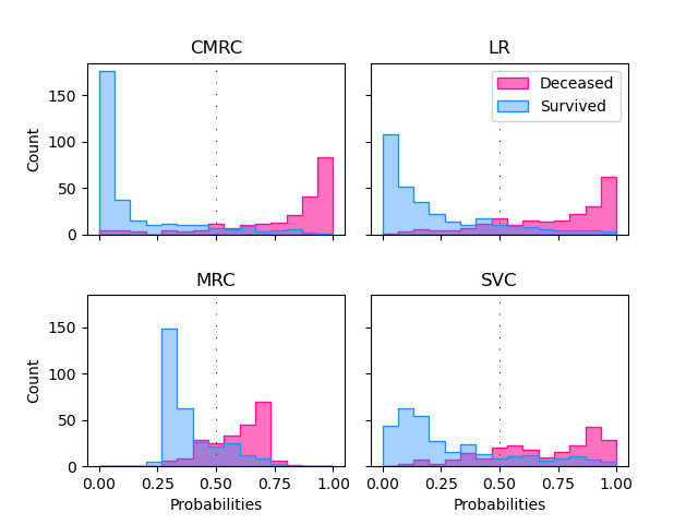
0.25 to 0.75. This estimation is very sensible to cut-off changes. The CMRC model shows a distribution where most of the cases are grouped around 0 and 1 for survive and decease respectively. This results are similar to the Logistic Regression’s but with less overlapping. SVC is the model with the worst performance of all having a lot of patients that survived with high decease probabilities.
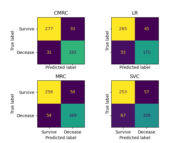
cm_cmrc = confusion_matrix(y_test, clf_CMRC.predict(X_test))  # CMRC
cm_mrc = confusion_matrix(y_test, clf_MRC.predict(X_test))  # MRC
cm_lr = confusion_matrix(y_test, clf_LR.predict(X_test))  # Logistic Regression
cm_svc = confusion_matrix(
    y_test, clf_SVC.predict(X_test)
)  # C-Support Vector Machine

fig, ax = plt.subplots(
    nrows=2,
    ncols=2,
    sharex="all",
    sharey="all",
    gridspec_kw={"wspace": 0, "hspace": 0.35},
)
ConfusionMatrixDisplay(cm_cmrc, display_labels=["Survive", "Decease"]).plot(
    colorbar=False, ax=ax[0, 0]
)
ax[0, 0].set_title("CMRC")
ConfusionMatrixDisplay(cm_mrc, display_labels=["Survive", "Decease"]).plot(
    colorbar=False, ax=ax[1, 0]
)
ax[1, 0].set_title("MRC")
ConfusionMatrixDisplay(cm_lr, display_labels=["Survive", "Decease"]).plot(
    colorbar=False, ax=ax[0, 1]
)
ax[0, 1].set_title("LR")
ConfusionMatrixDisplay(cm_svc, display_labels=["Survive", "Decease"]).plot(
    colorbar=False, ax=ax[1, 1]
)
ax[1, 1].set_title("SVC")
fig.tight_layout()
pd.DataFrame(
    classification_report(
        y_test,
        clf_CMRC.predict(X_test),
        target_names=["Survive", "Decease"],
        output_dict=True,
    )
).style.set_caption("Classification report CMRC").format(precision=3)
pd.DataFrame(
    classification_report(
        y_test,
        clf_MRC.predict(X_test),
        target_names=["Survive", "Decease"],
        output_dict=True,
    )
).style.set_caption("Classification report MRC").format(precision=3)
pd.DataFrame(
    classification_report(
        y_test,
        clf_LR.predict(X_test),
        target_names=["Survive", "Decease"],
        output_dict=True,
    )
).style.set_caption("Classification report LR").format(precision=3)
pd.DataFrame(
    classification_report(
        y_test,
        clf_SVC.predict(X_test),
        target_names=["Survive", "Decease"],
        output_dict=True,
    )
).style.set_caption("Classification report SVC").format(precision=3)
We can see in the classification reports and the confusion matrices the outperformance of CMRC.
Setting the cut-off point for binary classification:
In this section we will use beeswarm-boxplot to select the cut-off point to optimise the tradeoff between false positives and false negatives. The beeswarm-boxplot is a great tool to determine the performance of the model in each of the cases of the confusion matrix. On an ideal scenario the errors are located near the cut-off point and the true guesses are located near the 0 and 1 values.
fig, ax = plt.subplots(
    nrows=2,
    ncols=2,
    figsize=(10, 12),
    sharex="all",
    sharey="all",
    gridspec_kw={"wspace": 0.1, "hspace": 0.20},
)
scatterPlot(df_CMRC, ax[0, 0])
ax[0, 0].set_title("CMRC")
scatterPlot(df_MRC, ax[1, 0])
ax[1, 0].set_title("MRC")
scatterPlot(df_LR, ax[0, 1])
ax[0, 1].set_title("LR")
scatterPlot(df_SVC, ax[1, 1])
ax[1, 1].set_title("SVC")
plt.tight_layout()
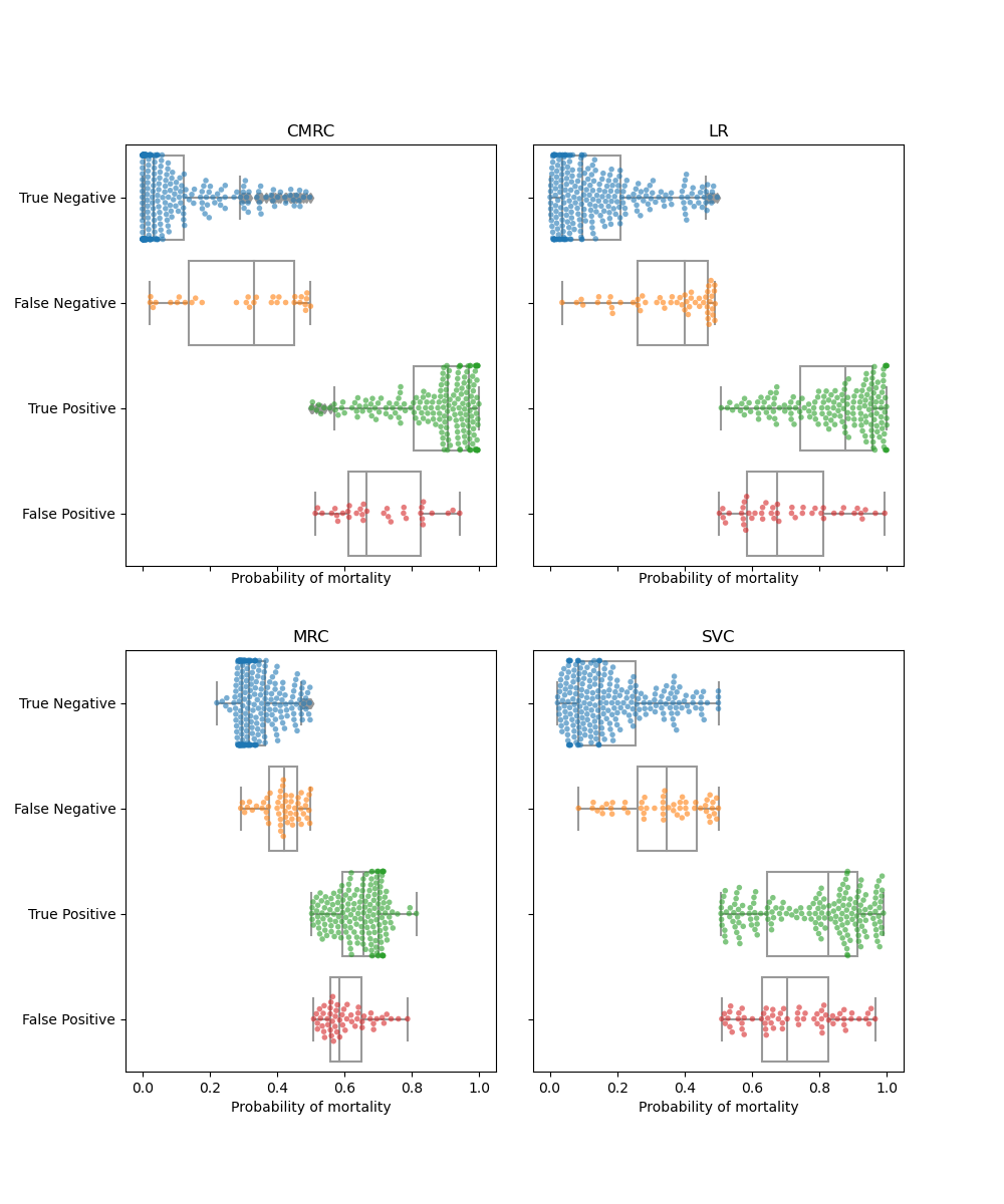
We see in the CMRC that the correct cases have a very good conditional probability estimation with around 75% of the cases very close to the extreme values. The most problematic cases are those with a low mortality probability estimation that had a fatal outcome (FN). In the CMRC model adjusting the threshold to 0.35 reduces the false negatives by 25% adding just some cases to the FP. In the MRC model adjusting the cutoff to 0.4 reduces half of the false negatives by trading of 25% of the TP.
threshold = 0.35
df_CMRC = defDataFrame(
    model=clf_CMRC, x_test=X_test, y_test=y_test, threshold=threshold
)
threshold = 0.4
df_MRC = defDataFrame(
    model=clf_MRC, x_test=X_test, y_test=y_test, threshold=threshold
)
pd.DataFrame(
    classification_report(
        df_CMRC.Real,
        df_CMRC.Prediction,
        target_names=["Survive", "Decease"],
        output_dict=True,
    )
).style.set_caption("Classification report CMRC \n adjusted threshold").format(
    precision=3
)
pd.DataFrame(
    classification_report(
        df_MRC.Real,
        df_MRC.Prediction,
        target_names=["Survive", "Decease"],
        output_dict=True,
    )
).style.set_caption("Classification report MRC \n adjusted threshold").format(
    precision=3
)
Comparing the outputs of this example we can determine that MRCs work significantly well for estimating the outcome of COVID-19 patients at hospital triage.
Furthermore, the CMRC model with threhsold feature mapping has shown a great performance both for classifying and for estimating conditional probabilities Finally we have seen how to select the cut-off values based on data visualization with beeswarm-boxplots to increase the recall in the desired class.
Total running time of the script: ( 0 minutes 0.000 seconds)